The first blog post in this series compared soybean, oil palm and olive using national harvested-area and production tables, then used CROPGRIDS to show where each crop is concentrated. That global grid is an effective screening layer: it covers 173 crops at 0.05° resolution, approximately 5.6 km at the equator.
This final use case changes the unit of analysis. Instead of asking where olive cultivation is concentrated in a global grid, we ask what can be learned when declared olive parcels are retained at their original field boundaries. We therefore move to EuroCrops V2, which harmonizes publicly released national crop declarations using the Hierarchical Crop and Agriculture Taxonomy (HCAT). The current release covers 16 EU Member States, represented by 18 national or regional data units; it does not currently provide parcel data for every EU country (Claverie et al., 2026). This restricted geographic coverage is the main trade-off for gaining a much finer, parcel-level analytical unit than CROPGRIDS.
The objective is not to estimate yield. It is to build a reproducible bridge from connected olive landscapes to comparable fields, and then test what the canopy-height product can reveal about canopy structure.
1. Finding connected olive landscapes
The preprocessing workflow retained 2023 EuroCrops parcels classified as olive in HCAT v4. Each field centroid was assigned to an H3 cell at resolution 10, and adjacent cells with the same crop class were grouped into connected components. H3 is an analytical connectivity layer; it does not replace the underlying EuroCrops field boundaries.
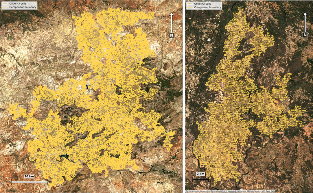
This produced 29,321 olive components larger than 15 ha. We ranked them by the summed area of their contributing fields. We selected the largest component in Spain, followed by the highest-ranked component belonging to a different country, which was in Portugal.
| Selected component | EuroCrops fields | H3 cells | Summed field area |
|---|---|---|---|
| Spain | 434,472 | 168,902 | 283,805.75 ha |
| Portugal | 11,111 | 5,346 | 4,818.00 ha |
The components can also be located within the Eurostat NUTS 2024 regional classification:
| Component | Broader region (NUTS 2) | Provincial or subregional coverage (NUTS 3) |
|---|---|---|
| Spain | Andalucía | Jaén, Córdoba, Granada and Málaga provinces |
| Portugal | Norte | Almost entirely Terras de Trás-os-Montes; two very small boundary fields fall in Alto Tâmega e Barroso |
These locations were assigned from the centroid of each contributing EuroCrops field. The Spanish component therefore represents a cross-province olive landscape rather than a single county or province. The Portuguese component is geographically more concentrated within northeastern Portugal.
The large difference in component size is itself informative. Connected-component rank identifies continuous concentrations under the chosen H3 rule; it does not create two landscapes of equal extent.
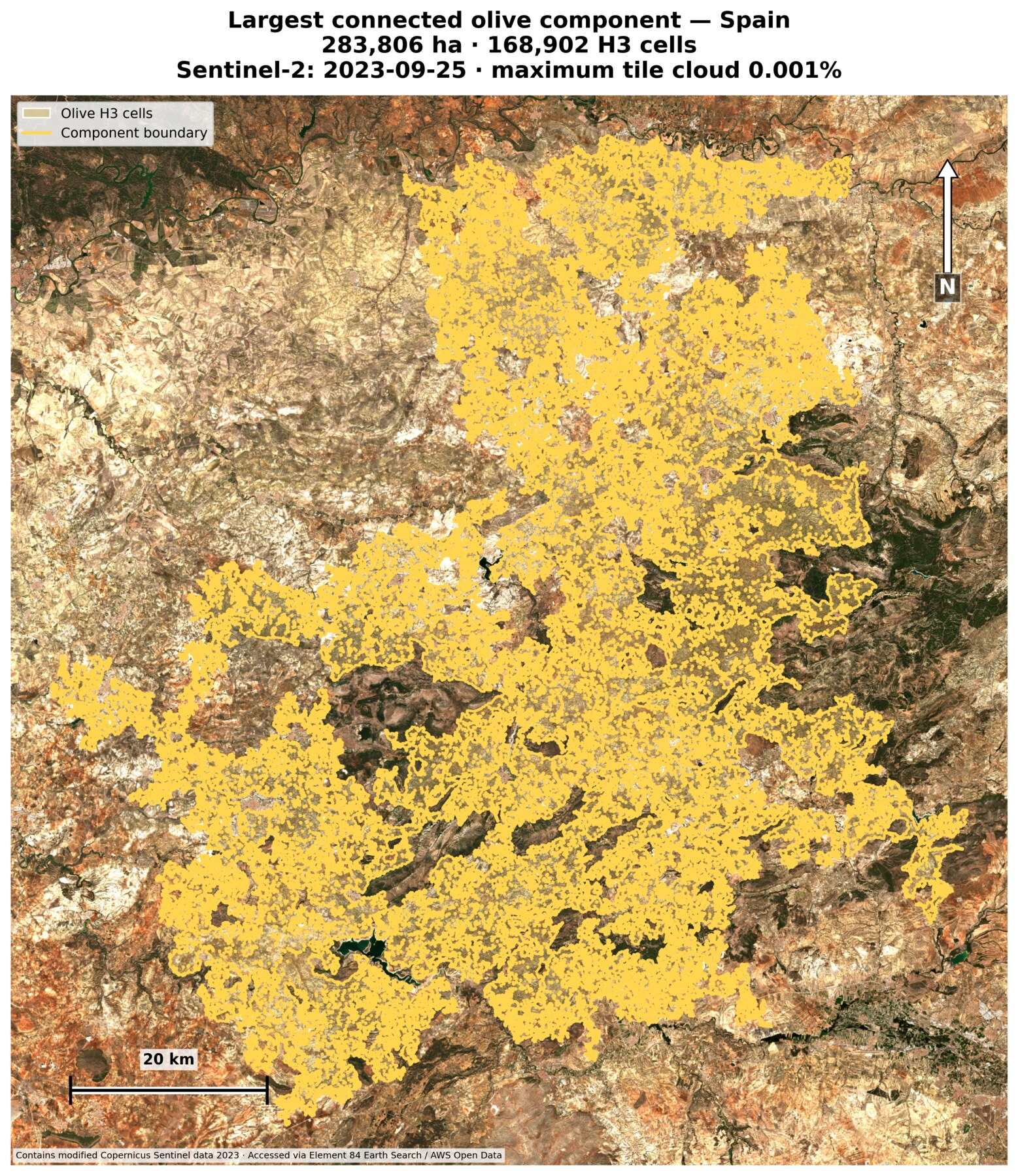
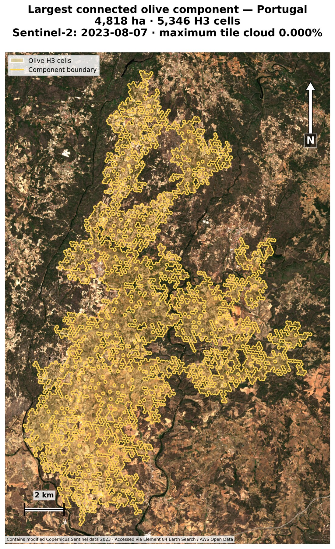
The static maps use cloud-free Sentinel-2 L2A true-colour scenes from 25 September 2023 in Spain and 7 August 2023 in Portugal. Sentinel-2 is used here only as visual context; the component membership comes from EuroCrops and H3.
Connected areas can support questions beyond crop output. They can help identify landscapes where coordinated monitoring, shared infrastructure, pest surveillance, fire planning or habitat-connectivity analysis may be useful. The definition remains sensitive to H3 resolution and the rule used to join neighbouring cells.
2. Returning from H3 cells to exact fields
The statistical comparison uses the exact EuroCrops polygons, not H3 hexagons. We retained fields of at least 1.5 ha and calculated five design variables for every eligible olive field in the two selected components:
- Exact field area: the area enclosed by the original EuroCrops parcel boundary, measured in hectares.
- Elevation midpoint: the midpoint between the field's 5th- and 95th-percentile elevations, used as a robust measure of its general elevation.
- Within-field elevation relief: the difference between those 5th- and 95th-percentile elevations, showing how much the terrain rises or falls inside the same field.
- 90th-percentile slope: a measure of the steeper parts of a field that is less sensitive to a few extreme pixels than the maximum slope.
- Polygon compactness: a shape measure distinguishing compact fields from long, narrow or irregular parcels.
These variables matter because a direct comparison could mix small hillside parcels with larger, flatter fields. After retaining only the field-size, terrain and shape groups represented in both components, the comparable population contained 10,718 Spanish fields and 491 Portuguese fields. A balanced, stratified sample of 250 fields per component was then selected using a fixed random seed.
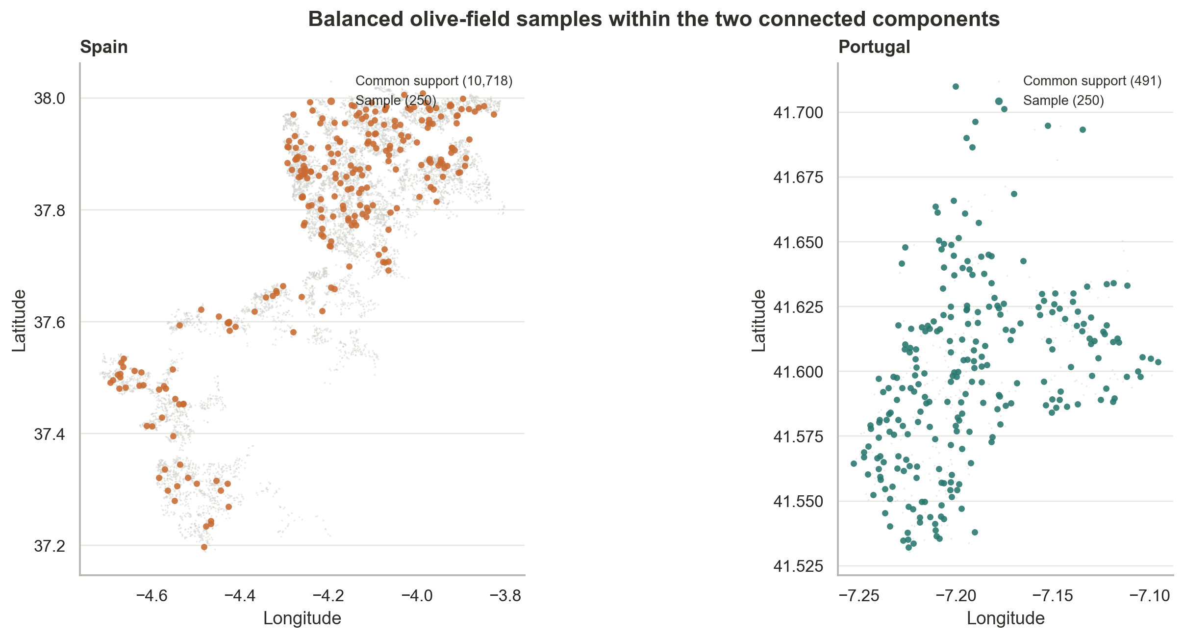
We checked balance using standardized mean differences. Before sampling, the two common-support populations still differed on several characteristics. After stratification and rerandomization, every absolute standardized difference was below the prespecified 0.15 threshold; the largest was 0.148.
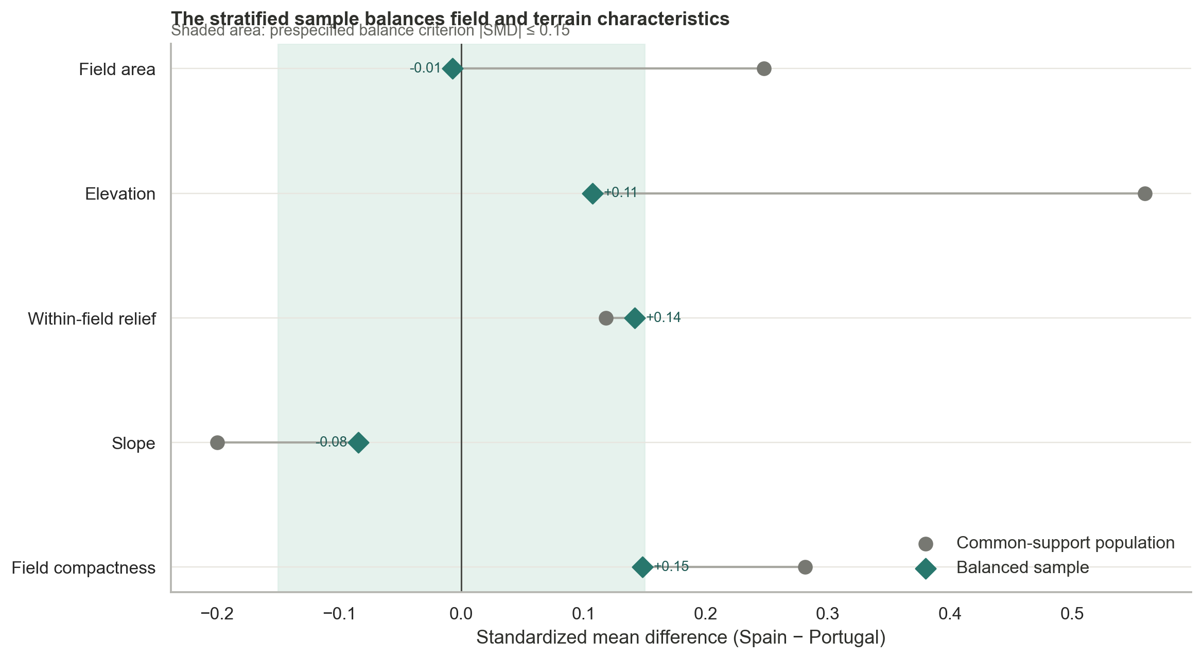
This design makes the sampled fields in the two selected areas more comparable, but it does not turn them into a national survey. The results describe these two connected olive-growing areas—not every olive field in Spain and Portugal. We also matched only characteristics available in the data: field size, elevation, relief, slope and shape. Other differences, such as cultivar, tree age, irrigation, pruning, farm management and local climate, were not measured and may still influence the comparison.
3. Connecting the fields to canopy height (CHMv2)
The previous oil-palm analysis used CHMv2 to examine canopy structure and candidate palm crowns within delineated plantation fields. We reuse that connection here, but olive groves present a more difficult test: crowns may be smaller, shorter, more irregular, closely spaced or partly merged in the modelled surface.
For every sampled field, we extracted CHMv2 within its original EuroCrops boundary. We calculated canopy-cover and canopy-height summaries, then applied the two-method, multi-spacing crown-candidate workflow used in the palm-oil analysis. The initial visibility screen required at least 95% valid CHMv2 coverage, at least 30 preliminary canopy peaks, at least 5% modelled canopy cover, and adequate peak contrast and spacing support. Fields passing that screen were then processed by the two-method ensemble; final verification required at least 10 accepted candidates and at least 50% agreement between the methods.
Before constructing the representative sample, five similarly sized Spanish–Portuguese field pairs were used as a visual check of the canopy-height data and exact parcel boundaries. These examples are illustrative only and do not contribute separate statistics to the component comparison.
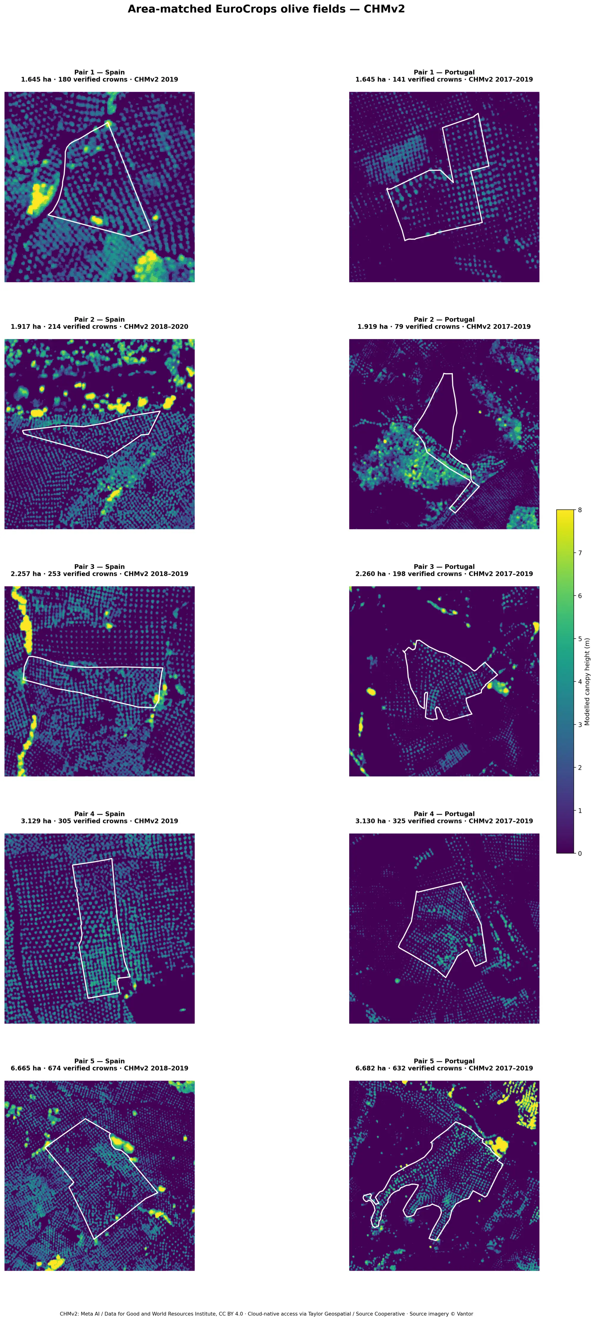
The distinction between tree, crown and crown candidate is important. CHMv2 is a modelled canopy-height surface, not a field inventory. A tree can be missed, fragmented into several peaks or merged with a neighbour. Candidate counts and nearest-neighbour distances are therefore algorithm outputs—not confirmed olive-tree counts or planting distances.
4. What differed between the two components (Spain, Portugal)?
The Spanish and Portuguese estimates were adjusted as if both samples contained the same proportions of the shared field-size, terrain and shape groups. This prevents a difference from being driven simply by one sample containing more fields from a particular group. To quantify uncertainty, we resampled complete field records 2,000 times, while preserving the sampling groups. For each statistic, the middle 95% of those repeated estimates forms its 95% confidence interval: narrower intervals indicate greater precision, while wider intervals indicate more uncertainty.
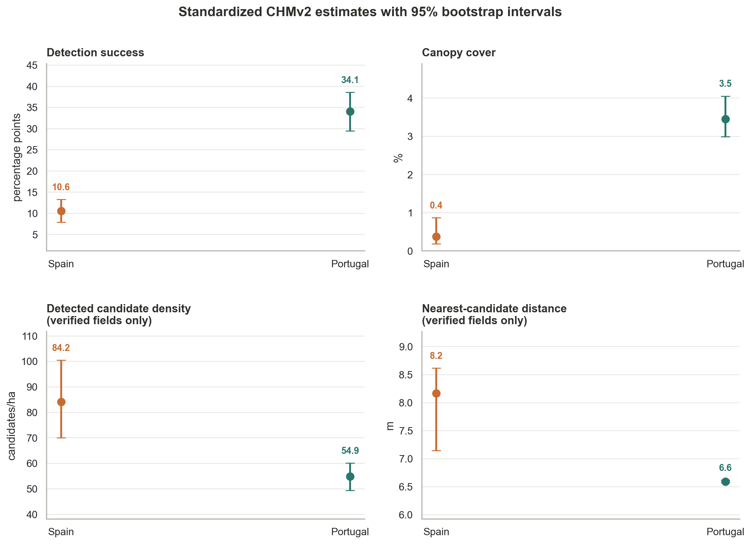
Four results stand out:
- Crown-candidate detection success: after adjustment, an estimated 10.6% of Spanish fields and 34.1% of Portuguese fields produced a canopy pattern that passed the full detection and agreement checks. Spain was therefore 23.5 percentage points lower (95% CI: −28.7 to −18.1). This result describes whether CHMv2 supported reliable candidate extraction in a field; it does not indicate that olive trees were actually absent.
- Modelled canopy cover: the median share of field pixels with a CHMv2 height of at least 1.5 m was 0.38% in Spain and 3.45% in Portugal. Spain was 3.08 percentage points lower (95% CI: −3.60 to −2.43). Low cover may reflect genuinely sparse or low vegetation, but it may also indicate canopy that the model did not resolve.
- Detected candidate density: among fields that passed verification, the median was 84.2 candidates/ha in Spain and 54.9 candidates/ha in Portugal. Spain was higher by 29.3 candidates/ha (95% CI: 14.5 to 43.3). This comparison applies only to the successfully detected subset and must not be generalized to every sampled field.
- Candidate nearest-neighbour distance: among fields with a resolvable candidate pattern, the median distance from each detected candidate to its closest neighbour was 8.17 m in Spain and 6.59 m in Portugal. Spain was 1.57 m higher (95% CI: 0.55 to 2.02). This is spacing between model-detected canopy peaks—not confirmed planting distance between olive-tree trunks.
The candidate-density comparison is based on 26 Spanish fields and 85 Portuguese fields that passed the complete verification. The nearest-neighbour comparison uses the 28 Spanish and 90 Portuguese fields that passed the initial visibility screen. The large difference in the number of usable fields is therefore part of the result: CHMv2 produced canopy patterns suitable for candidate analysis much more often in the Portuguese sample. The density and distance findings describe only those usable subsets.
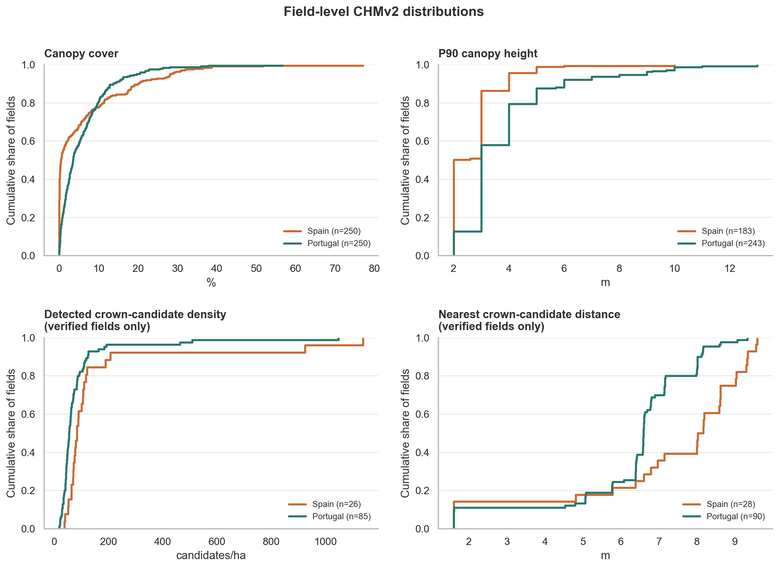
The combination of lower detection success but higher candidate density in Spain is not contradictory. Fewer Spanish fields produced a resolvable crown pattern, but the fields that did pass contained more detected peaks per hectare. Because this density result applies only to the successfully detected subset, it does not prove that the Spanish component has denser olive planting overall.
5. What this can—and cannot—say about production
The earlier article reported 2023 national production-to-harvested-area ratios of 1.92 t/ha for Spain and 3.14 t/ha for Portugal. Those values motivated the question of whether grove structure might differ, but the present analysis does not explain that national contrast.
Production per harvested hectare can also respond to rainfall, temperature, humidity, frost, drought, soil-water availability, irrigation, cultivar, grove age, pruning, alternate bearing, pests, harvest method and reporting practice. A stronger yield study would require spatially and temporally aligned production observations plus weather and management covariates. The CHMv2 source imagery also spans different acquisition periods across the two components, so component and observation date cannot be separated here.
The production-to-harvested-area difference is not visible or testable from this sample, because the sampled fields contain no measured harvest or production records. The defensible conclusion is therefore narrower: after making the sampled fields more comparable in size, terrain and shape, CHMv2 showed different canopy detectability and modelled canopy patterns in the two connected olive landscapes. These differences are worth investigating, but they cannot be presented as the reason for the national production-per-hectare difference.
Together, the sources demonstrate why scale matters: CROPGRIDS identifies the global concentration, H3 exposes landscape continuity, EuroCrops preserves the declared field, and CHMv2 adds a canopy-level measurement layer.
Attribution:
- EuroCrops field boundaries and crop labels: EuroCrops V2, provided by the European Commission Joint Research Centre and contributing national administrations. The current release covers 16 EU Member States rather than the entire EU. The polygons are agricultural declarations rather than independently surveyed cadastral boundaries.
- Sentinel-2 context imagery: Contains modified Copernicus Sentinel data 2023, accessed through Element 84 Earth Search. The imagery provides visual context and was not used to assign crop type.
- Terrain variables: Copernicus DEM GLO-30, used to derive field elevation, within-field relief and slope.
- Canopy height: Meta and World Resources Institute, 2026, Version 2 High Resolution Canopy Height Maps (CHMv2), licensed under CC BY 4.0. Cloud-native access was provided through Taylor Geospatial Engine Labs and Source Cooperative. Source imagery for CHMv2 © Vantor. Acquisition periods vary between the selected fields.
- Derived components, samples and crown candidates: H3 components, balanced samples, canopy summaries and candidate crown centres were generated for this analysis. Crown candidates are remote-sensing detections and are not field-verified olive-tree inventories.
- Series connection: Previous Monopteryx post on soybean, oil palm and olive crop grids and field-level oil-palm analysis.
Monopteryx connects crop declarations, field geometry and Earth-observation products to create reproducible landscape and parcel-level evidence.